Fragmentation and dissolution rates

Fragmentation rate \(k_\text{frag}\) and dissolution rate \(k_\text{diss}\) control the rate at which polymer mass is lost from particle size classes, either to smaller size classes (fragmentation) or dissolved organics (dissolution). They have units of inverse time (s^-1 in SI units) and thus, for a given period of time \(t + \Delta t\), a mass \(m = \Delta t k_{i,t}\) of polymer fragments or dissolves from size class \(i\). The Fragment size distribution controls how this mass is split amongst daughter size classes.

Both rate constants can vary in time and across particle surface areas, and thus they are 2D arrays with dimensions (n_timesteps, n_size_classes). This dependence is controlled by the parameters provided in model input data, specifically to the k_frag and k_diss variables. If scalars are provided to these, the rates are constant in time and surface area, and if a dict of regression parameters is provided, the rate constants vary in time and surface area according to these parameters, as detailed here.

The rate constant distributions are built using either a compound relationship:

\[ k(t,s) = k_f T(t) S(s) + k_0 \]

or an additive relationship:

\[ k(t,s) = k_f (T(t) + S(s)) + k_0 \]

You can specify which is used by specifying the boolean is_compound in the k_frag or k_diss input data dict. Here, t is the time dimension, s is the particle surface area dimension, k_f is the rate constant scaling factor, k_0 is the rate constant baseline adjustment factor and k could be k_frag or k_diss. T(t) is the expression used to create the time-dependence distribution, and S(s) the surface area distribution. Both of these take the same form, which allows for power law, exponential, logarithmic and logistic regressions:

\[ X(x) = A_x \hat{x}^{\alpha_x} \cdot B_x e^{-\beta_x \hat{x}} \cdot C_x \ln (\gamma_x \hat{x}) \cdot \frac{D_x}{1 + e^{-\delta_{x,1}(\hat{x} - \delta_{x,2})}} \]

or if the user specifies a list for parameter \(A_x\), a polynomial instead of power law can be used:

\[ X(x) = \sum_{n=1}^N A_{x,n} \hat{x}^n \cdot B_x e^{-\beta_x \hat{x}} \cdot C_x \ln (\gamma_x \hat{x}) \cdot \frac{D_x}{1 + e^{-\delta_{x,1}(\hat{x} - \delta_{x,2})}} \]

Here, X(x) is either T(t) or S(s). The parameters A_t, A_s, alpha_t etc are the parameters provided to the k_frag and k_diss dicts in the input data. The dimension value \(\hat{x}\) is normalised such that the median value is equal to 1: \(\hat{x} = x/\tilde{x}\), where \(\tilde{x}\) is the median of \(x\). This ensures regressions are not skewed by t and s values that are many orders of magnitude apart.

Smallest size class

The model presumes that no fragmentation happens from the smallest size class, and so k_frag is always set to 0 for this size class. This is in constast to dissolution, which can happen from this size class.

Regression parameters

Parameter	Type, default	Description
k_f	Float, required	Rate constant scaling factor
k_0	Float, default=0	Rate constant baseline adjustment factor
A_t, A_s	Float or list, default=1	Power law coefficient. If a scalar is provided, this is used as the coefficient for a power law expression with alpha_x as the exponent. If a list is provided, these are used as coefficients in a polynomial expression, where the order of the polynomial is given by the length of the list. For example, if a length-2 list A_t=[2, 3] is given, then the resulting polynomial will be 3*t**2 + 2*t (note the list is in ascending order of polynomials).
alpha_t, alpha_s	Float, default=0	If A_x is a scalar, alpha_x is the exponent for this power law expression. For example, if A_t=2 and alpha_t=0.5, the resulting power law will be 2*t**0.5.
B_t, B_s	Float, default=1	Exponential coefficient
beta_t, beta_s	Float, default=0	Exponential scaling factor
C_t, C_s	Float or None, default=None	If a scalar is given, this is the coefficient for the natural logarithmic term. If None is given, the logarithmic term is set to 1 (i.e. it is ignored).
gamma_t, gamma_s	Float, default=1	Logarithmic scaling factor
D_t, D_s	Float or None, default=None	If a scalar is given, this is the coefficient for the logistic term. If None is given, the logistic term is set to 1.
delta1_t, delta1_s	Float, default=1	Logistic growth rate (steepness of the logistic term)
delta2_t, delta2_s	Float or None, default=None	Midpoint of the logistic curve, which denotes the t or s value where the logistic curve is at its midpoint. If None is given, the midpoint is assumed to be the at the midpoint of the t or s range. For example, if the model timesteps go from 1 to 100, then the default for delta2_t is 50.
is_compound	Bool, default=True	Whether the t and s regression terms should be combined by multiplying them together (compound) or adding them. Choice depends on whether you think the time- and size-dependence of rate constants affect each other or act independently.

Negative k values

Make sure to specify regression parameters that do not end up in negative k values. The model checks for these before running and will throw a FMNPDistributionValueError exception if any are found.

Examples

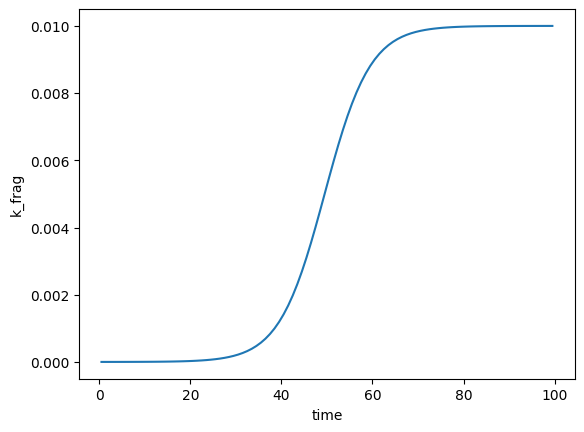
The make this more understandable, here are some examples are how you might use these parameters in real life. The first thing to note is that, if you want a k distribution to follow one particular regression, such as logistic, then you only need to specify parameters for that regression and the defaults take care of making sure the other regressions are constant. Taking a logistic regression as an example for k_frag:

import numpy as np
import matplotlib.pyplot as plt
from fragmentmnp import FragmentMNP
from fragmentmnp.examples import minimal_config, minimal_data

# By specifying D_t=1, we are telling the model that we want a
# logistic regression over time for k_frag. delta1_t controls
# the steepness of the logistic
minimal_data['k_frag'] = {
    'k_f': 0.01,
    'D_t': 1,
    'delta1_t': 10
}

# Init the model with these data, which generates the k distributions
fmnp = FragmentMNP(minimal_config, minimal_data)

# Plot the k_frag distribution to check that it is logistic. We
# didn't specify any surface area dependence params and so we
# can pick any size class except the smallest (which always 
# has k_frag=0)
plt.plot(fmnp.t_grid, fmnp.k_frag[1, :])
plt.xlabel('time')
plt.ylabel('k_frag')

Text(0, 0.5, 'k_frag')

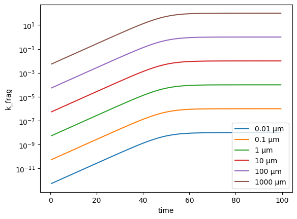
In the above, we effectively specified that k_frag should follow the regresion \(k_\text{frag} = 0.01 / (1 + e^{-(\hat{t} - 1)})\). Let’s now introduce a linear surface area dependence. Because the particle size classes are log-spaced, we plot with a log yscale in order to see the fragmentation rates for the smaller size classes:

# Specify a logistic regression over t and linear over s
minimal_data['k_frag'] = {
    'k_f': 0.01,
    'D_t': 1,
    'delta1_t': 10,
    'A_s': [0.01]
}

# Init the model
fmnp = FragmentMNP(minimal_config, minimal_data)

# Plot k_frag for all size classes except the smallest
plt.plot(fmnp.t_grid, fmnp.k_frag[1:, :].T)
plt.legend([f'{c * 1e6:<1g} µm' for c in fmnp.psd[1:]])
plt.xlabel('time')
plt.ylabel('k_frag')
plt.yscale('log')

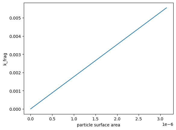
We can double check that the surface area dependence is linear by plotting the surface area against k_frag for one timestep:

plt.plot(fmnp.surface_areas[1:], fmnp.k_frag[1:, 0])
plt.xlabel('particle surface area')
plt.ylabel('k_frag')

Text(0, 0.5, 'k_frag')

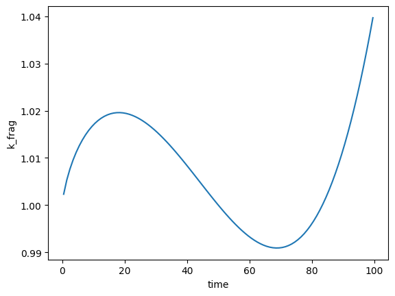
Combining regressions can make for some weird and wonderful distribution shapes:

# Third-order polynomial combined with a logarithmic regression - why not!?
minimal_data['k_frag'] = {
    'k_f': 0.01,
    'k_0': 1,
    'A_t': [-5, -2, 3],
    'C_t': 1
}
# Create and plot
fmnp = FragmentMNP(minimal_config, minimal_data)
plt.plot(fmnp.t_grid, fmnp.k_frag[1, :])
plt.xlabel('time')
plt.ylabel('k_frag')

Text(0, 0.5, 'k_frag')

Setting your own \(k_\text{frag}\) array

If the time and size dependencies that can be achieved using the regression parammeters above are not flexible enough for your scenario, you can of course set your own \(k_\text{frag}\) or \(k_\text{diss}\) arrays by modifying the k_frag or k_diss attributes directly after initialising the model:

# Set a random k_frag array (really?!)
fmnp.k_frag = np.random.rand(fmnp.n_size_classes, fmnp.n_timesteps)