Fragmentation rate¶

The fragmentation rate \(k_\text{frag}\) is arguably the most important model parameter, describing the rate at which the mass of polymer in each size class fragments. It has units of s^-1 and thus, for a given period of time \(t + \Delta t\), a mass \(m = \Delta t k_\text{frag,i,t}\) of polymer fragments from size class \(i\). The Fragment size distribution controls how this mass is split amongst daughter size classes.

Fragmentation is size class and time dependent, and thus internally is a 2D array of dimensions (n_timesteps, n_size_classes). The size class dependence is controlled by input parameter theta_1 (\(\theta_1\)) and the time dependence by k_frag_tau (\(\tau\)):

\[ k_{\text{frag},i,t} = k_\text{frag,av} \cdot \frac{d_i^{2 \theta_1} \cdot t^\tau}{d_\text{median}^{2 \theta_1} \cdot t_\text{median}^\tau} \]

where \(k_\text{frag,av}\) is the scalar input parameter k_frag (note a size-dependent distribution can also be input), \(d\) is the size class diameter and \(t\) is the timestep index (which is 1-indexed). The median diameter and timestep index are used such that \(k_\text{frag,av}\) represents the (unweighted) average fragmentation rate across size and time.

We can test what this dependence looks like in practice by using the model to calculate this fragmentation rate array:

from fragmentmnp import FragmentMNP
from fragmentmnp.examples import minimal_config, minimal_data

# Set an arbitrary average fragmentation rate, theta_1 and tau
minimal_data['k_frag'] = 0.1
minimal_data['theta_1'] = -0.001
minimal_data['k_frag_tau'] = -0.001

# Create a new model instance used these
fmnp = FragmentMNP(minimal_config, minimal_data)
fmnp.k_frag.shape

(100, 7)

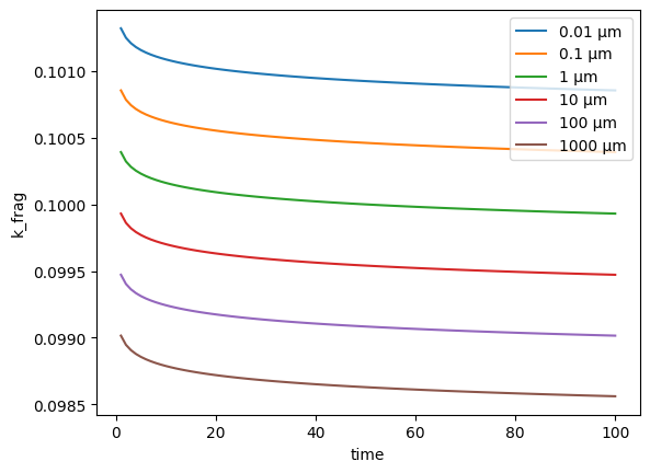
The minimal_config sets n_timesteps to 100 and n_size_classes to 7, and hence the shape of the k_frag array is (100, 7). Let’s plot this dependence:

import numpy as np
import matplotlib.pyplot as plt

def plot_k_frag(fmnp):
    # Plot the time evolution of the fragmentation rate for
    # each size class. We exclude the smallest size class as
    # this always has k_frag=0
    plt.plot(np.arange(1, fmnp.n_timesteps + 1), fmnp.k_frag[:,1:])
    plt.legend([f'{c * 1e6:<1g} µm' for c in fmnp.psd[1:]])
    plt.xlabel('time')
    plt.ylabel('k_frag')

plot_k_frag(fmnp)

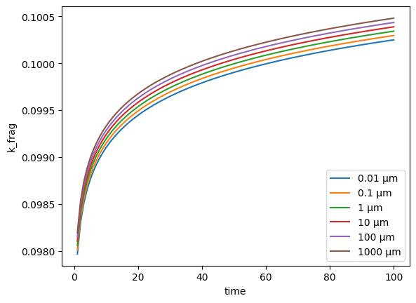
As you can see, setting a negative theta_1 and k_frag_tau means that the fragmentation rate decreases with increasing time and particle diameter. Now if we update theta_1 and k_frag_tau to be positive, we will see the inverse depedence. We also change the values to show a strong time dependence but weaker size dependence:

minimal_data['theta_1'] = 0.0001
minimal_data['k_frag_tau'] = 0.005
fmnp = FragmentMNP(minimal_config, minimal_data)
plot_k_frag(fmnp)

Setting your own \(k_\text{frag}\) array¶

If the time and size dependencies that can be achieved using \(\theta_1\) and \(\tau\) are not suitable for your application, you can of course set your own \(k_\text{frag}\) array by modifying the k_frag attribute directly after initialising the model:

# Set a random k_frag array (really?!)
fmnp.k_frag = np.random.rand(fmnp.n_timesteps, fmnp.n_size_classes)

FRAGMENT-MNP

Fragmentation rate

Contents

Fragmentation rate¶

Setting your own \(k_\text{frag}\) array¶